An Introduction To Formal Logic
Preamble
This blog is a personal study of formal logic, philosophy, and mathematics. It aims to formalize various classical and modern philosophical works in a variety of formal logic systems, both weak and strong. I have decided to use Lean for these formalizations. I have no degree in these fields but I hope it will be of high enough quality to be of interest to scholars, both amateur and professional.
An Introduction to Formal Logic
What is logic?
It is a system of reasoning using rules, with the goal of determining truth. Formal logic uses a language with a formal grammar. This allows us to look more closely at philosophical discussions in a manner akin to mathematics; formal logic is indeed a part of mathematics. The grammar and rules are the syntax of the language, the meaning of the rules is the semantics. When syntactic provability aligns with semantic truth, the system is sound: no matter how you interpret it, the logic makes sense. When every possible truth is provable, the system is complete. Gödel proved first-order logic complete in 1929, before turning around in 1931 and proving that any system capable of arithmetic is incomplete; mathematicians have been a fantastic source of revenue for psychotherapists as a result of the existential crises this causes.
To illustrate the difference between syntax and semantics, let's examine the turnstile and the double turnstile.
\vdash \Phi
This single turnstile means "\Phi (Phi) is derivable from the axioms"
\models \Phi
This double turnstile means "\Phi is true in all interpretations"
But further, let's look at it in Lean. Lean is built around the turnstile, this block of code is essentially declaring \vdash P \to P (you can derive from the axioms of the system that if P is true then P is true - a trivial example).
example (P : Prop) : P → P := P:Prop⊢ P → P
P:Prophp:P⊢ P
All goals completed! 🐙
The idea of the double turnstile is a level above this - but we can discuss it when we look at metalogic in Lean much later.
The structure of logic
Logic, especially in formal logic systems, has a hierarchy of building blocks, starting from the most basic concepts and layering on top of these.
Propositions
The simplest element is the proposition. A proposition is simply a name for some thing with a truth value. We could use "The sky is blue" as a proposition and name it something like S. Or we could use "Triangles have four sides" and call it T - though we generally won't use T because it looks a lot like \top, also called top / True. Convention at the most basic level of propositional logic is to use capital letters P, Q, R, S, etc. Note that the first proposition (the sky is blue) seems obviously true and the second proposition seems obviously false - that's fine. Propositions aren't always true, they just have a truth value. However, propositions aren't nonsensical statements like "all things that are aren't sometimes." The useful thing about propositions is that the rules of logic apply regardless of what that meaning is. This allows us to analyze the structure of a discussion to determine if it is logically valid without getting into the mess of the exact meaning of the proposition.
We've got Propositions in Lean:
variable (P : Prop)
Here we just declare that there is a proposition P. We know nothing else about it, not even what it means. You'll notice this resembles declaring a variable in various programming languages. That's because it is (more correctly due to the Curry-Howard correspondence it's a Type, which we'll get into later). It can be helpful to think of propositions like variables. They have a value, and what that value is will determine how they act within a derivation.
Connectives
Propositions by themselves are pretty boring. All of math and logic is pretty boring if you just look at the objects (also it's boring in general for some people). The magic happens in the relationships between objects (category theory nerds' ears just perked up). Connectives are logical operators that can be combined with propositions to make what is called Well Formed Formulas (WFF).
A well formed formula is either a proposition or a well-formed formula connected with connectives. You can (and we often will) nest WFFs.
In natural deduction systems, connectives have introduction and elimination rules that allow us to determine when and how we can add them or remove them when performing our inference.
Let's look at the commonly used connectives for Propositional Logic, the simplest system and the foundation for everything else.
Conjunction
Conjunction uses the symbol \land, and it's a binary infix operator (it goes in between propositions, just like + does when adding numbers). We read it aloud as "and", and if you're familiar with programming you've almost certainly used and in your if-then-else blocks. P \land Q is read as "P and Q"; it allows us to treat the combination of P and Q as its own proposition, one which is only true if both P and Q are true.
Let's look at it in Lean:
#eval decide (True ∧ True) -- true
#eval decide (True ∧ False) -- false
#eval decide (False ∧ True) -- false
#eval decide (False ∧ False) -- false
-- a simple example --
example (P Q : Prop) (hp : P) (hq : Q) : P ∧ Q := ⟨hp, hq⟩
The first four lines there demonstrate the behavior with various proposition values. The example can be read as "Example: for Propositions P and Q, assuming we have a proof of P (called hp) and a proof of Q (called hq), we can prove P \land Q using hp and hq".
Disjunction
No points awarded for guessing this next connective. It's disjunction, and it uses the symbol \lor. This symbol is read aloud as "or", and you've probably already guessed how it works; it connects two propositions into one value that is true if either proposition is true (or both). It's also a binary infix operator much like conjunction.
A similar quick look in Lean:
#eval decide (True ∨ True) -- true
#eval decide (True ∨ False) -- true
#eval decide (False ∨ True) -- true
#eval decide (False ∨ False) -- false
-- We only need to prove P or Q --
example (P Q : Prop) (hp : P) : P ∨ Q := Or.inl hp
example (P Q : Prop) (hq : Q) : P ∨ Q := Or.inr hq
Here our examples are a bit different: we only need to prove one of the propositions to be able to prove the disjunction of the two propositions. This is why if you have an obligation to mail a letter, you have an obligation to mail a letter or burn a letter. Don't worry about that example too much we'll cover it when we get to deontic logic. Disjunctions can be said to "weaken" an expression: the claim being proven is a weaker claim that at least one of the propositions is true.
Implication
I had a joke here but it sucked so I deleted it. I have mercifully spared you the experience.
Let's talk implications. They're written with an arrow \to, binary infix again like P \to Q and they're read as "if P then Q" or "P implies Q". This connective is the bread and butter of logical inference. You're going to see it everywhere.
If you're used to programming in various languages above a surface level, you'll recognize this as a function. Mathematically it can be considered a function as well, with various results according to the theory you use (set theory for example has functions which sends the elements of a set to the elements in its codomain.) For you engineers, this is a function that is called with arguments and returns a return value. If your language has the guts, you'll even know that each of these arguments has a type and the return value has a type. If it's got even more guts the function will have a type. You might even have generics, which is cool. Lean 4 fully supports dependent types, so, y'know. It's kinda cool like that. This means in Lean we can fully explore the way different parts of mathematics are the same as each other in some very cool and useful ways. When pieces of Math are the same thing viewed from different angles it's called "duality." The fact that these particular aspects of mathematics and type theory correspond - that propositions are types - is called the Curry-Howard correspondence. This very important fact means that we can do a lot of high-quality math work very reliably because mathematical proofs are programs. Working in Lean, we get to see this aspect of the literal laws of reality laid bare before us. It's some seriously cool stuff on a cosmic level.
However, we're starting at the basics with propositional logic. Let's look at how implication works, using Lean to demonstrate it.
#eval decide (True → True) -- true
#eval decide (True → False) -- false
#eval decide (False → True) -- true
#eval decide (False → False) -- true
-- Modus ponens: if we have P → Q and P, we get Q
example (P Q : Prop) (h : P → Q) (hp : P) : Q := P:PropQ:Proph:P → Qhp:P⊢ Q
P:PropQ:Proph:P → Qhp:P⊢ P
All goals completed! 🐙
-- Identity: P implies P
example (P : Prop) : P → P := P:Prop⊢ P → P
P:Prophp:P⊢ P
All goals completed! 🐙
-- Weakening: from P we can derive Q → P
example (P Q : Prop) : P → Q → P := P:PropQ:Prop⊢ P → Q → P
P:PropQ:Prophp:P⊢ Q → P
P:PropQ:Prophp:Phq:Q⊢ P
All goals completed! 🐙
I think of particular interest is the truth evaluations; it's almost certainly going to surprise at least one software engineer to see the statement #eval decide (False → True) evaluate to True. This is an important aspect of this connective: something can be true with its condition being false - it's not exactly like an if-then statement that you might be used to. Let's look at it in natural language. We might say "if it is raining then the grass outside is wet", and this would be represented perhaps as Raining \to WetGrass or R \to W. The entire statement "if it is raining then the grass outside is wet" is what we are considering the truth value of. It's entirely possible for the grass outside to be wet (W true) while it is not raining (R false) if for example the lawn irrigation system were active. At the same time, it's still true that if it is raining then the grass outside is wet, even though it is not currently raining.
It's for a similar reason to disjunction that we can weaken any proposition by adding an additional proposition to its left. In natural language we could consider it like taking the proposition "the sky is blue" and prepending another proposition: "if the moon has disappeared then the sky is blue." This statement isn't necessarily true, but because the sky is in fact blue it doesn't matter what we put in front of it; it nicely mirrors the quite literal "one of these options is true" meaning of disjunction as this is quite mechanically "if P then Q" with a side of "Q can happen some other way."
Negation
Our next logical connective to discuss is negation. Negation uses the symbol \neg and can be said aloud "not". It's a pretty simple idea and operates how you would expect, but it's also notably our first unary prefix operator
#check Not -- Prop → Prop
#print Not -- fun a => a → False
-- Truth evaluations
#eval decide (¬True) -- false
#eval decide (¬False) -- true
-- If we have P and ¬P, we get anything (explosion)
example (P Q : Prop) (hp : P) (hnp : ¬P) : Q := absurd hp hnp
It's important to understand here that True and False in propositional logic are different from the idea of Boolean values. True and False, which can be written \top and \bot (sometimes called "top" and "bottom" for the reason that in a lattice these are the maximum and minimum element, respectively) represent a different concept than programmers might initially intuit. To say that a propositional variable like P is \top is to declare it provable. To say that a propositional variable P is \bot is to declare it contradictory or otherwise impossible.
Biconditional
The biconditional is sometimes called "equivalence", though that can represent a different concept. It is written \leftrightarrow and said aloud "if and only if"; it is sometimes written "iff" or \iff or \equiv. A quick look in Lean:
#eval decide (True ↔ True) -- true
#eval decide (True ↔ False) -- false
#eval decide (False ↔ True) -- false
#eval decide (False ↔ False) -- true
-- Biconditional is two implications
example (P Q : Prop) (hpq : P → Q) (hqp : Q → P) : P ↔ Q :=
⟨hpq, hqp⟩
The biconditional P \iff Q is essentially a statement that (P \to Q) \land (Q \to P).
Inference Rules
Having covered propositions and connectives, we've covered the entire alphabet available to us and we're now ready to play with logic. But before we get anywhere we need to understand the rules of the game. Much like a board game, we have legal and illegal moves, defined in the inference rules of the system we use. It's a little backwards to discuss rules before discussing how to write and evaluate proofs, but I think it's actually a more intuitive way to discuss these things.
Essentially, when we start a proof we start with axioms. Statements assumed to be true. This could even be nothing, if we really feel like it. Then from these axioms, we can introduce and eliminate formulas using inference rules.
We're going to be doing this in Lean itself, because we might as well start working in something that lets us check our work. In Lean you begin a proof by introducing a goal - this is our win condition.
theorem trivial_theorem : True := ⊢ True
-- At this point, goal is: top
All goals completed! 🐙 -- True is trivially true!
#check trivial_theorem
This can be read as "we call this theorem the 'trivial theorem', we can prove True by the trivial example."
When you're working on a theorem, and you're pretty sure but you can't exactly prove a theorem yet, you can "just" use the sorry tactic:
theorem fermats_last_theorem :
(n : Nat) → 2 < n → ¬∃ (a b c : Nat), a > 0 ∧ b > 0 ∧ c > 0 ∧ a^n + b^n = c^n := ⊢ ∀ (n : Nat), 2 < n → ¬∃ a b c, a > 0 ∧ b > 0 ∧ c > 0 ∧ a ^ n + b ^ n = c ^ n
All goals completed! 🐙
#check fermats_last_theorem
This reads as "We call this theorem 'Fermat's last theorem', we can prove that for any natural number n greater than two there do not exist three natural numbers greater than 0 (a, b, c) such that:
a^n + b^n = c^n
and we can prove this by.... Sorry, I've got a proof of this but there isn't room in the margin here.
That will check! You can start theorems this way and start breaking them apart
Conjunction Rules
Welcome back to \land land. Let's check out its introduction and elimination rules. Introduction can be thought of as a constructor used in programming because that's exactly what it is. For you still stuck in Object-oriented languages who just can't get out of that mindset, you can think of it like the constructor of a class, which produces an instance of the class. That's similar to (but still very different from) a function that constructs a term of a type. This idea is made pretty explicit with the constructor tactic in Lean:
theorem and_intro (P Q : Prop) (hp : P) (hq : Q) : P ∧ Q := P:PropQ:Prophp:Phq:Q⊢ P ∧ Q
-- Goal: P ∧ Q
P:PropQ:Prophp:Phq:Q⊢ PP:PropQ:Prophp:Phq:Q⊢ Q
-- Goal 1: P
P:PropQ:Prophp:Phq:Q⊢ Q
-- Goal 2: Q
All goals completed! 🐙
This can be read as: we have a theorem called and_intro where P and Q are propositions. Suppose P is true, let's call the example of this hp, and suppose Q, again calling this hypothetical idea (a hypothesis if you will, and that's literally what's it's called here) hq. We want to construct P \land Q - to do that we need to show both P and Q. Hey, we've got the hypothesized P and Q right here!
Put more simply, it states "If You have P and Q then you may introduce P \land Q.
Now let's look at elimination.
theorem and_elim_left (P Q : Prop) (h : P ∧ Q) : P := P:PropQ:Proph:P ∧ Q⊢ P
-- Goal: P
cases h with
P:PropQ:Prophp:Phq:Q⊢ P All goals completed! 🐙
-- Conjunction Elimination Right: extract Q from P ∧ Q
theorem and_elim_right (P Q : Prop) (h : P ∧ Q) : Q := P:PropQ:Proph:P ∧ Q⊢ Q
-- Goal: Q
cases h with
P:PropQ:Prophp:Phq:Q⊢ Q All goals completed! 🐙
Conjunction has right and left elimination rules - what's elimination? That's how we use up a statement. Just like we introduced P \land Q we eliminate the \land and we can get P and Q from it. This means, "If you've got P \land Q then you can get P and you can get Q. Note the hypothesis in this case is "suppose P \land Q we'll call this h." Then we use the cases tactic, which deconstructs our hypothesis h into hp and hq - and then in the two different examples we just gesture to one or the other
Sorry that's incredibly boring actually. Am I actually going to just list introduction and elimination rules for all the logical connectives in propositional logic? Yes! But let's spice it up with some abstract nonsense. Strap in.
You always have to say it when using Category Theory so here goes: a monad is a monoid in the category of endofunctors. Secondly, categories: categories consist of objects (equipped with unique identity morphisms) and morphisms between objects, from domain to codomain. There can be any count of objects in a category, and any count of morphisms between them. Several axioms apply:
-
Composition: For morphisms
f: a \to b,g: b \to cthere is a morphismg \circ f: a \to c -
Associativity: For the morphisms
f: a \to b,g: b \to c,h: c \to d,(h \circ g) \circ f = h \circ (g \circ f) -
Identity: For the morphisms
f: a \to b,f \circ id_a = f = id_b \circ f
A morphism is called an isomorphism when it has an inverse morphism so that you can traverse bidirectionally, for the example morphisms f: a \to b and g: b \to a, f \circ g = id_b and g \circ f = id_a
You now understand Category Theory. Here's a Group, as a treat.
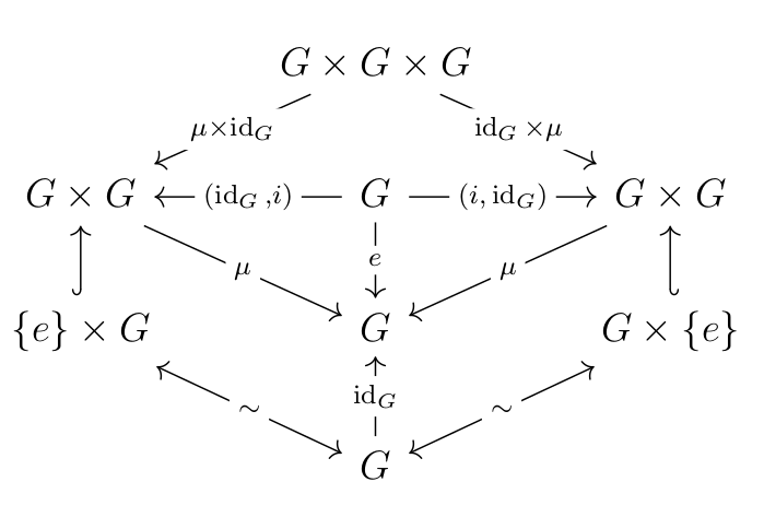
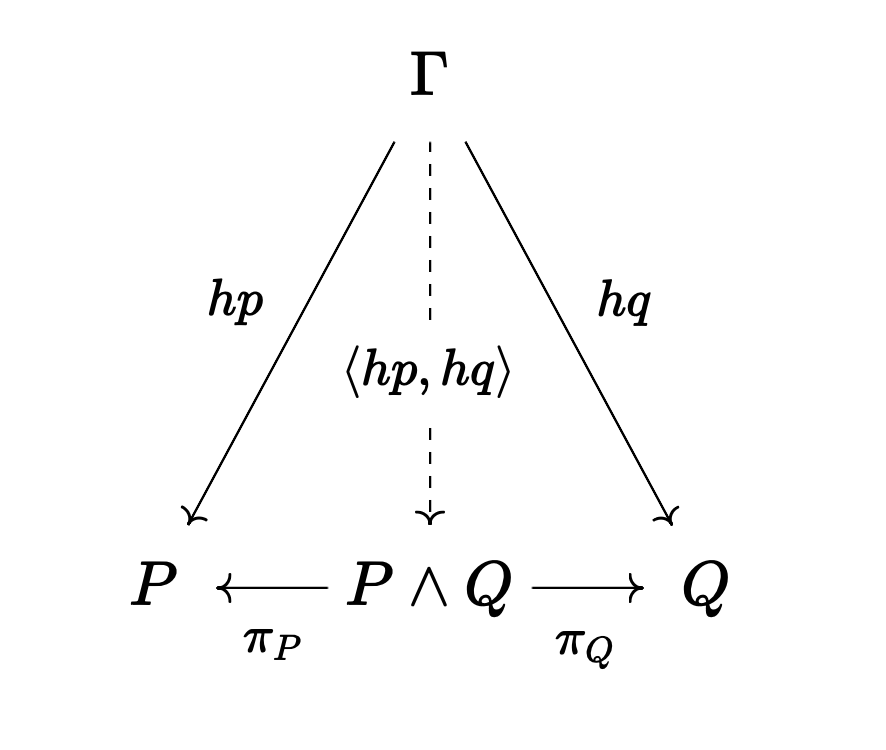
In propositional logic, all the connectives can be represented by universal objects, and the morphisms into the object are the introduction rules and the morphisms out of the object are the elimination rules. For example, conjunction is a categorical product:
Let's speed run the rest. I've got ADHD, stimulants, and really interesting set of ideas for my next posts.
Disjunction Rules
Disjunction is the dual of conjunction, and this is reflected in its introduction and elimination rules which exactly mirror the conjunction with two introduction rules and one elimination rule.
theorem or_intro_left (P Q : Prop) (hp : P) : P ∨ Q := P:PropQ:Prophp:P⊢ P ∨ Q
-- Goal: P ∨ Q
P:PropQ:Prophp:P⊢ P
All goals completed! 🐙
-- Disjunction Introduction Right: Q gives P ∨ Q
theorem or_intro_right (P Q : Prop) (hq : Q) : P ∨ Q := P:PropQ:Prophq:Q⊢ P ∨ Q
-- Goal: P ∨ Q
P:PropQ:Prophq:Q⊢ Q
All goals completed! 🐙
-- Disjunction Elimination: case analysis on P ∨ Q
theorem or_elim (P Q R : Prop) (h : P ∨ Q) (hpr : P → R) (hqr : Q → R) : R := P:PropQ:PropR:Proph:P ∨ Qhpr:P → Rhqr:Q → R⊢ R
-- Goal: R
cases h with
P:PropQ:PropR:Prophpr:P → Rhqr:Q → Rhp:P⊢ R All goals completed! 🐙
P:PropQ:PropR:Prophpr:P → Rhqr:Q → Rhq:Q⊢ R All goals completed! 🐙
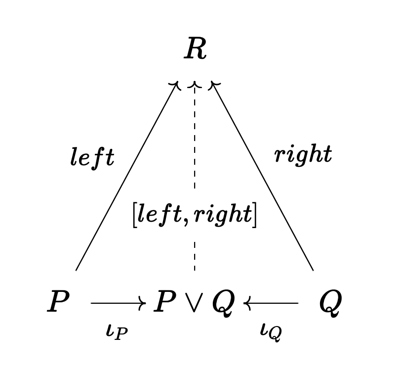
A disjunction is a coproduct, the categorical dual of the product. A product in a category C is a coproduct in C^{op} - it is a contravariant functor applied to the diagram.
Implication Rules
Implication is a... complicated concept to describe. Type-theoretically it is introduced via a lambda abstraction - a definition of a function. It is eliminated through function application.
theorem impl_intro (P Q : Prop) (h : P → Q) : P → Q := P:PropQ:Proph:P → Q⊢ P → Q
-- Goal: P → Q
P:PropQ:Proph:P → Qhp:P⊢ Q
All goals completed! 🐙
-- Implication Elimination: modus ponens
theorem impl_elim (P Q : Prop) (h : P → Q) (hp : P) : Q := P:PropQ:Proph:P → Qhp:P⊢ Q
-- Goal: Q
All goals completed! 🐙
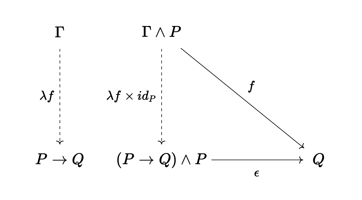
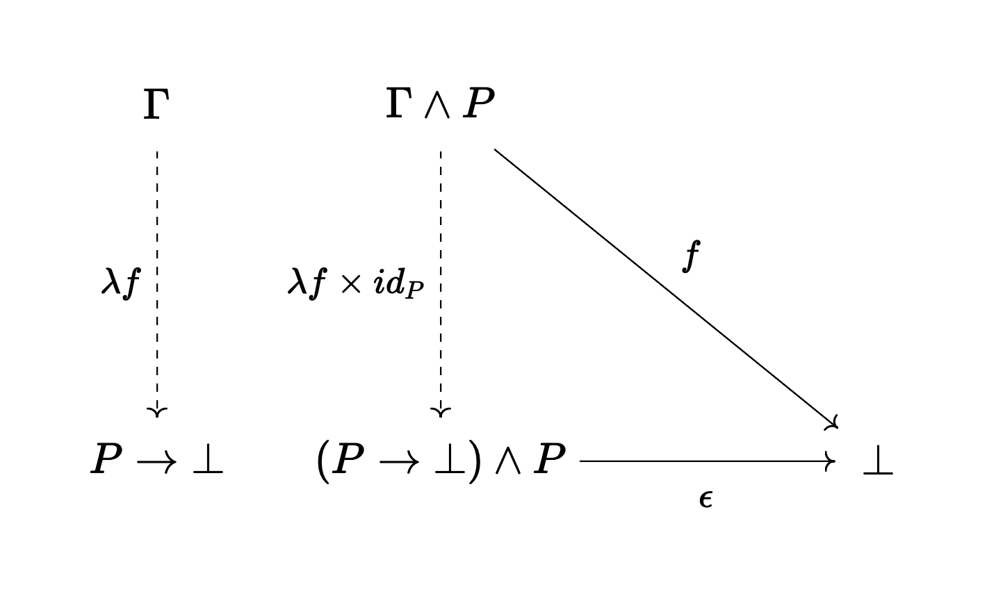
Categorically speaking this is an exponential object. In this diagram we "curry" the morphism f:(\Gamma \land P) \to Q. This morphism represents the ability to reach Q if we add P to the context \Gamma. The exponential transpose is the morphism \lambda f: \Gamma \to (P \to Q) that packages this proof of Q given P into an exponential object P \to Q. The morphism \epsilon: ((P \to Q) \land P) \to Q is the evaluation morphism - the elimination rule, modus ponens.
Negation Rules
Negation is very interesting. Here it is in Lean.
theorem neg_intro (P : Prop) (h : P → False) : ¬P := P:Proph:P → False⊢ ¬P
-- Goal: ¬P
All goals completed! 🐙
-- Negation Elimination: explosion (ex falso quodlibet)
theorem neg_elim (P Q : Prop) (hp : P) (hnp : ¬P) : Q := P:PropQ:Prophp:Phnp:¬P⊢ Q
-- Goal: Q
All goals completed! 🐙
Surprise! It's just an exponential again!
Biconditional Rules
This one is really complicated so if I really feel like it I'll come back here and cover it. Here's Lean:
theorem iff_intro (P Q : Prop) (hpq : P → Q) (hqp : Q → P) : P ↔ Q := P:PropQ:Prophpq:P → Qhqp:Q → P⊢ P ↔ Q
-- Goal: P ↔ Q
P:PropQ:Prophpq:P → Qhqp:Q → P⊢ P → QP:PropQ:Prophpq:P → Qhqp:Q → P⊢ Q → P
P:PropQ:Prophpq:P → Qhqp:Q → P⊢ Q → P
All goals completed! 🐙
-- Biconditional Elimination Left: forward direction
theorem iff_elim_left (P Q : Prop) (h : P ↔ Q) : P → Q := P:PropQ:Proph:P ↔ Q⊢ P → Q
-- Goal: P → Q
All goals completed! 🐙
-- Biconditional Elimination Right: backward direction
theorem iff_elim_right (P Q : Prop) (h : P ↔ Q) : Q → P := P:PropQ:Proph:P ↔ Q⊢ Q → P
-- Goal: Q → P
All goals completed! 🐙
Categorically, it's a product of exponentials. Can you imagine me drawing that diagram? I would, but I'm currently dealing with two kids with RSV while "vacationing" in Wisconsin for Christmas. Self care and all that.
But I've got a much cooler post coming up next.
A teaser: robots in disguise.